Graph的特征表示非常复杂:
1.复杂的拓扑结构,较难从图像中的感受野提取有效信息;
2.无特定的节点顺序;
3.通常graph会是动态变化的, 且使用多模态特征。
高质量的节点表征能够用于衡量节点的相似性,同时高质量的节点表征也是准确分类节点的前提。
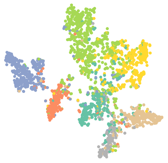
本文以Cora论文引用网络数据集为例,对MLP、GCN、GAT三种神经网络的分类性能进行对比。首先载入数据集并定义可视化函数:
1 | #载入数据集 |
1 | #定义可视化函数,并观察整体数据分布 |
1. MLP(Multi-layer Perceptron)在图节点分类中的应用
多层感知机(MLP,Multilayer Perceptron)也叫人工神经网络(ANN,Artificial Neural Network).
1.1 MLP代码
1 | #构造MLP |
结果:
MLP(
(lin1): Linear(in_features=1433, out_features=16, bias=True)
(lin2): Linear(in_features=16, out_features=7, bias=True)
)
该MLP由两个线性层、一个ReLU非线性层和一个dropout组成。第一个线程层将1433维的节点表征嵌入(embedding)到低维空间中(hidden_channels=16),第二个线性层将节点表征嵌入到类别空间中(num_classes=7)。
1 | #训练MLP |
结果:
Epoch: 050, Loss: 1.1777
Epoch: 100, Loss: 0.5491
Epoch: 150, Loss: 0.4577
Epoch: 200, Loss: 0.2876
1 | #测试训练后的MLP |
结果:
Test Accuracy: 0.5850
MLP的结果较差,是因为用于训练此神经网络的有标签节点数量过少,它对未见过的节点泛化能力很差。
2 GCN(Graph Convolutional Network)在图节点分类中的应用
GCN,图卷积神经网络,本质上和CNN的作用一样,就是一个特征提取器,只不过它的对象是图数据。关键在于如何定义局部感受域:
- Spatial approach: 指定节点的边的方向;
- Spectral approach: 通过图的拉普拉斯矩阵的特征值和特征向量对图结构进行处理.
2.1 GCN公式
$$
\mathbf{X}^{\prime} = \mathbf{\hat{D}}^{-1/2} \mathbf{\hat{A}}\mathbf{\hat{D}}^{-1/2} \mathbf{X} \mathbf{\Theta}
$$
其中$\mathbf{\hat{A}} = \mathbf{A} + \mathbf{I}$表示插入自环的邻接矩阵,$\mathbf{I}$是单位矩阵,$\hat{D}{ii} = \sum{j=0} \hat{A}{ij}$表示$\mathbf{\hat{A}}$的对角线度矩阵。$\mathbf{\hat{D}}^{-1/2} \mathbf{\hat{A}}
\mathbf{\hat{D}}^{-1/2}$是对称归一化矩阵,它的节点式公式为:
$$
\mathbf{x}^{\prime}i = \mathbf{\Theta} \sum{j \in \mathcal{N}(v) \cup{ i }} \frac{e{j,i}}{\sqrt{\hat{d}_j \hat{d}i}} \mathbf{x}j
$$
其中,$\hat{d}i = 1 + \sum{j \in \mathcal{N}(i)} e{j,i}$,$e{j,i}$表示从源节点$j$到目标节点$i$的边的对称归一化系数(默认值为1.0)。
2.2 GCN代码
1 | #构造GCN |
结果:
GCN(
(conv1): GCNConv(1433, 16)
(conv2): GCNConv(16, 7)
)
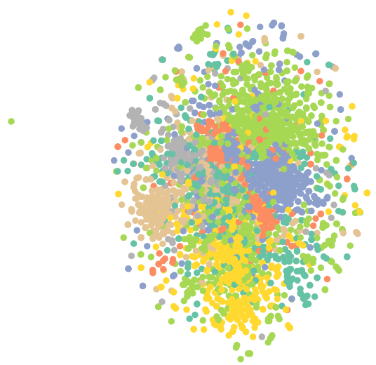
1 | #可视化未训练的GCN |
1 | #训练GCN |
结果:
Epoch: 050, Loss: 1.1346
Epoch: 100, Loss: 0.5471
Epoch: 150, Loss: 0.4021
Epoch: 200, Loss: 0.3391
1 | #测试 |
结果:Test Accuracy: 0.8090
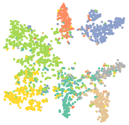
1 | #可视化训练后的GCN |
3.GAT(Graph Attention Network)在图节点分类中的应用
GAT的提出解决了GCN存在的问题:
- GCN 假设图是无向的,因为利用了对称的拉普拉斯矩阵 (只有邻接矩阵 A 是对称的,拉普拉斯矩阵才可以正交分解),不能直接用于有向图。
- GCN 不能处理动态图,GCN 在训练时依赖于具体的图结构,测试的时候也要在相同的图上进行。因此只能处理 transductive 任务,不能处理 inductive 任务。
- GCN 不能为每个邻居分配不同的权重,GCN 在卷积时对所有邻居节点均一视同仁,不能根据节点重要性分配不同的权重。
3.1 GAT公式
图注意力算子:
$$
\mathbf{x}^{\prime}i = \alpha{i,i}\mathbf{\Theta}\mathbf{x}{i} +
\sum{j \in \mathcal{N}(i)} \alpha_{i,j}\mathbf{\Theta}\mathbf{x}{j}
$$
注意力系数$\alpha{i,j}$为:
$$
\alpha_{i,j} =
\frac{
\exp\left(\mathrm{LeakyReLU}\left(\mathbf{a}^{\top}
[\mathbf{\Theta}\mathbf{x}_i , \Vert , \mathbf{\Theta}\mathbf{x}j]
\right)\right)}
{\sum{k \in \mathcal{N}(i) \cup { i }}
\exp\left(\mathrm{LeakyReLU}\left(\mathbf{a}^{\top}
[\mathbf{\Theta}\mathbf{x}_i , \Vert , \mathbf{\Theta}\mathbf{x}_k]
\right)\right)}
$$3.2 GAT代码
1
2
3
4
5
6
7
8
9
10
11
12
13
14
15
16
17
18
19
20
21
22
23#构造GAT
import torch
from torch.nn import Linear
import torch.nn.functional as F
from torch_geometric.nn import GATConv
class GAT(torch.nn.Module):
def __init__(self, hidden_channels):
super(GAT, self).__init__()
torch.manual_seed(2021)
self.conv1 = GATConv(dataset.num_features, hidden_channels)
self.conv2 = GATConv(hidden_channels, dataset.num_classes)
def forward(self, x, edge_index):
x = self.conv1(x, edge_index)
x = x.relu()
x = F.dropout(x, p=0.5, training=self.training)
x = self.conv2(x, edge_index)
return x
model = GAT(hidden_channels=16)
print(model)结果:
GAT((conv1): GATConv(1433, 16, heads=1) (conv2): GATConv(16, 7, heads=1))
1
2
3
4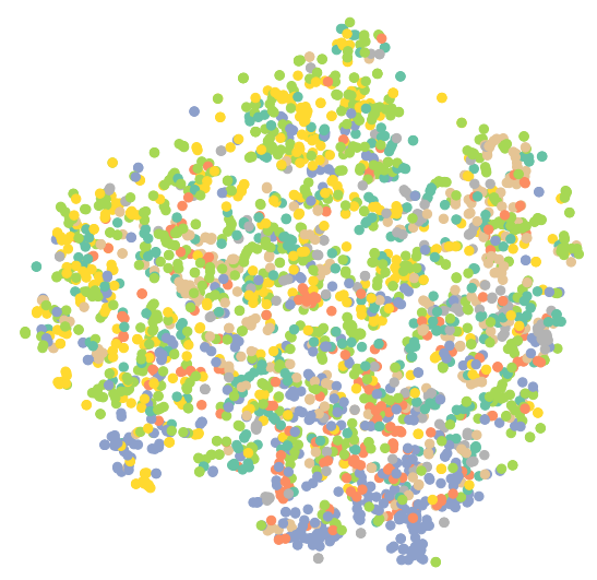
5#可视化未训练的GAT
model.eval()
out = model(data.x, data.edge_index)
visualize(out, color=data.y)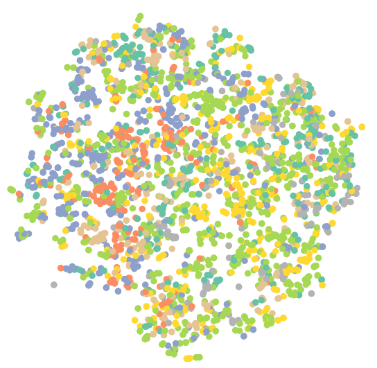
1 | #训练GAT |
结果:
Epoch: 050, Loss: 0.8583
Epoch: 100, Loss: 0.3209
Epoch: 150, Loss: 0.2267
Epoch: 200, Loss: 0.1939
1 | #测试GAT |
结果:Test Accuracy: 0.7310
1 | #可视化训练后的GAT |
4.总结
GCN和GAT的结果都优于MLP,原因是他们同时考虑了节点自身信息与周围邻接节点的信息.
GCN和GAT的共同点:
- 都遵循消息传递范式;
- 在邻接节点信息变换阶段,它们都对邻接节点做归一化和线性变换;
- 在邻接节点信息聚合阶段,它们都将变换后的邻接节点信息做求和聚合;
- 在中心节点信息变换阶段,它们都只是简单返回邻接节点信息聚合阶段的聚合结果。
GCN和GAT的不同点在于归一化方法不同():
- GCN根据中心节点与邻接节点的度计算归一化系数;GAT根据中心节点与邻接节点的相似度计算归一化系数。
- GCN的归一化方式依赖于图的拓扑结构:不同的节点会有不同的度,同时不同节点的邻接节点的度也不同,于是在一些应用中GCN图神经网络会表现出较差的泛化能力;GAT的归一化方式依赖于中心节点与邻接节点的相似度,相似度是训练得到的,因此不受图的拓扑结构的影响,在不同的任务中都会有较好的泛化表现。
参考资料
1.datawhale-GNN开源学习资料
2.知乎-图节点表征学习
3.GCNConv官方文档
4.GATConv官方文档
5.GAT图注意力网络
